Randomizing 3 rows of text across columns in Google Sheets

This post will show a method I used to get 3 columns of data to randomize across the columns. That is, data stays within its row, but scatters across columns. 

Using these formulas, a list of text will automatically be randomized like this:

Randomizing rows of text across columns in Google Sheets

I'll explain what I ended up doing, or you can scroll down to the end for a direct summary. 

Background

A teacher friend came to me with an interest request. He wanted to make a test worksheet for little kids, where they choose "Which of these is the ___?" He had lists of 3 types of words, arranged in columns by type of words, but he wanted them mixed in order to make random answer choices.

For example, he had lists like this which he had taught the kids:

Animals	Plants	Toys
Dog	Rose	Teddy Bear
Cat	Oak Tree	Lego
Elephant	Tulip	Barbie Doll
Lion	Grass	Action Figure
Giraffe	Sunflower	Puzzle
Monkey	Pine Tree	Toy Car
Horse	Dandelion	Board Game
Rabbit	Cactus	Dollhouse
Bird	Fern	Play-Doh
Fish	Maple Tree	Stuffed Animal

That's a real HTML table, so in case it doesn't appear right, here it is in image form:

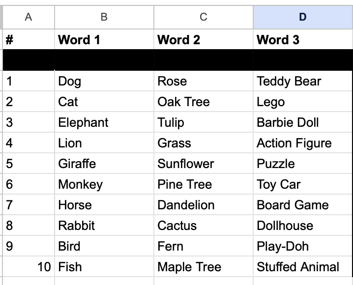Table of ESL vocab, organized into 3 columns

But he wanted them mixed up so he could make simple questions on worksheets. Questions like:

Which of the following are animals?

Q1:     Rose        Teddy Bear        Dog

Q2:     Lego        Cat                Oak Tree

Desired "output": randomized choices from the columns

You get the idea.

Problem with the Google Sheets "Randomize" function: by columns, not rows

The problem he was having is that using the default "Randomize" function inside Google Sheets, data is kept organized by column rather than row, so that if he selected the entire range of text, choosing Randomize would still keep all animals in the animal column, all plants in the plant column, etc. 

Randomize range option

Randomized position within the columns, but not across the rows

This behavior is not ideal. since now his worksheet would have all answers as answer choice "A".

So, knowing that I know stuff about computers, he contacted me asking if I knew a way to do what he wanted to do.

I'll be honest, I thought I could just select each individual row one-by-one, and run the Randomize function, expecting that to force Sheets to randomize their placement in the row. That would be a pain in the butt, but a Macro could be used to make Sheets do the repetitive work. Or based on how often he will need this, just do it by hand. But I was annoyed to discover that there is no Randomize function if you highlight only a row:

Randomize range function grayed out when trying to randomize by rows

Looks like this would be harder than I thought, and reminded me of the old programmers adage: "We do this not because it is easy, but because we thought it would be easy."

After playing around with this for way longer than I had anticipated due to not wanting to injury my pride as a "computer guy," I finally came up with a solution.

Now I won't claim that this is the most efficient or ideal solution to the problem, but this worked. And "it works" usually means "good enough" where I'm from. 

Preliminary thinking: Randomly generate 6 situations

I focused on the idea that randomizing 3 sets of words would result in 6 possible outcomes. Assuming all the animal words are A, plant words are B, toy words are C, then they could be arranged like this:

1. ABC
2. ACB
3. BAC
4. BCA
5. CAB
6. CBA

So I figured I could try something like this:

1. Generate a random number at each row (Google Sheets has a formula for this).
2. Divide the resulting number value into 6 chunks
3. Assign an ABC "situation" to each resulting chunk
4. Based on the resulting "situation", arrange the 3 cells accordingly

For mental simplicity, I made the random number (which is always between 0 and 1) multiplied so that it would be a whole number between 1 and 100. 

So now, if my random number comes out between 1 and 17, that's an "ABC situation." If it comes out between 17 and 33, that's a "ACB situation" and so on. 

I probably could have skipped this whole 3-letter combination thing and made a formula directly extrapolating from the random number, but this made it easier to think about conceptually. 

So I first wanted to make a formula that would achieve this.

Solution (Part 1): "Situational" IFS formula

This took some trial and error, since I had to combine multiple conditions with "AND" formulas. The AND formulas were simply because I didn't know another way to achieve the "if the random number is between 17 and 33" syntax. I tried 17<X<33 but that didn't seem to work.

For my own sake, I decided to rename the 6 of the ABC, ACB... situations into A1, A2, B1, B2, C1, C2.

So, I combined multiple AND conditions into a single IFS formula, like so:

=IFS(AND(F3 >= 0, F3 <= 17), "A1",

     AND(F3 >= 17, F3 <= 33), "A2",

     AND(F3 >= 33, F3 <= 50), "B1",

     AND(F3 >= 50, F3 <= 67), "B2",

     AND(F3 >= 67, F3 <= 84), "C1",

     AND(F3 >= 84, F3 <= 100), "C2")

It loos like a lot, and it is a lot, but I only need do make this once in a single column after my random number generator, then fill-down the rest of the rows. 

I could have combined this too into the random number generator, but again it's easier for me to conceptualze them separately. 

This ends up printing the "situation" type next to my random number generator. Remember, these "situations" are just mental constructs for me. I know that, for example, if the random number is 70, that will now equate to situation C1. 

Mentally, I know that C1 = CAB = Word 3 Word 1 Word 2.

Adding the formula to column G and filling down, I can see that it's working.

Random numbers equating to certain "situation" types

So now, based on what kind of "situation" appears here, I will have 3 new columns display their contents appropriately. 

Solution (Part 2): IFS formulas for the cells

So next, I drew up 3 IFS formulas for the 3 columns that basically say:

1. If this row is situation A1, display Word 1 here. 
2. If it's situation A2, display Word 1 here.
3. If it's situation B1, display Word 2 here...

And so on for all 6 types of situations. The only change I need for each row is the references cells (the words).

So 1st column formula:

=IFS(G3="A1",B3,G3="A2",B3,G3="B1",C3,G3="B2",C3,G3="C1",D3,G3="C2",D3)

2nd column formula:

=IFS(G3="A1",C3,G3="A2",D3,G3="B1",B3,G3="B2",D3,G3="C1",B3,G3="C2",C3)

3rd column formula:

=IFS(G3="A1",D3,G3="A2",C3,G3="B1",D3,G3="B2",B3,G3="C1",C3,G3="C2",B3)

Then fill-down. 

The result is that these 3 columns grab the words from the list (which haven't been tampered with at all!) according to the "situation" made by the random number generator.

Columns I, J, and K pull in words from Columns B, C, D depending on the "situation".

Here, Situation B2 calls for Word 2 (rose) to be displayed in I, Word 3 (teddy bear) in J, and Word 1 (dog) in K.

Filling down meant that each cell in Column I is checking the situation listed in Column G, and displaying the contents of Columns B,C,D in which ever order is prescribed by that "situation."

I know this looks complex, and I wish I could think of a better way of doing it, but now that this is all set up, it can be reused and/or expanded forever. 

Summary - just give me the final formulas!

Here's what my table content would look like as plain text (no formulas obviously in the HTML)

#	Word 1	Word 2	Word 3		Rand	Situation		Rand A	Rand B	Rand C
1	Dog	Rose	Teddy Bear		52	B2		Rose	Teddy Bear	Dog
2	Cat	Oak Tree	Lego		31	A2		Cat	Lego	Oak Tree
3	Elephant	Tulip	Barbie Doll		97	C2		Barbie Doll	Tulip	Elephant
4	Lion	Grass	Action Figure		18	A2		Lion	Action Figure	Grass
5	Giraffe	Sunflower	Puzzle		5	A1		Giraffe	Sunflower	Puzzle
6	Monkey	Pine Tree	Toy Car		50	B1		Pine Tree	Monkey	Toy Car
7	Horse	Dandelion	Board Game		99	C2		Board Game	Dandelion	Horse
8	Rabbit	Cactus	Dollhouse		29	A2		Rabbit	Dollhouse	Cactus
9	Bird	Fern	Play-Doh		33	A2		Bird	Play-Doh	Fern
10	Fish	Maple Tree	Stuffed Animal		27	A2		Fish	Stuffed Animal	Maple Tree

And an image:

The full table I'm using

Based on the image above, you can recreate this by adding the fomulas:

Cell F3

=RAND()*100

---

Cell G3

=IFS(AND(F3 >= 0, F3 <= 17), "A1",

     AND(F3 >= 17, F3 <= 33), "A2",

     AND(F3 >= 33, F3 <= 50), "B1",

     AND(F3 >= 50, F3 <= 67), "B2",

     AND(F3 >= 67, F3 <= 84), "C1",

     AND(F3 >= 84, F3 <= 100), "C2")

---

Cell I3

=IFS(G3="A1",B3,G3="A2",B3,G3="B1",C3,G3="B2",C3,G3="C1",D3,G3="C2",D3)

---

Cell J3

=IFS(G3="A1",C3,G3="A2",D3,G3="B1",B3,G3="B2",D3,G3="C1",B3,G3="C2",C3)

---

Cell K3

=IFS(G3="A1",D3,G3="A2",C3,G3="B1",D3,G3="B2",B3,G3="C1",C3,G3="C2",B3)

That will get you the identical Google Sheet that I ended up sharing with him. 

Final thoughts

From there, he can now easily extract the randomized word choices. To make simple A. B. C. answer choices, he can add another column before each one and fill those down. He can freely copy/paste that in a Google Doc or Word Document. 

And it's done. I wish Sheets had this ability built-in. What if he ever wants to make 4 possible answer choices? I suppose if the order of the rows (the order within each column) isn't important, then he could break up the columns and do a few basic Randomizings and paste the chunks back together, but that would make strings of "right" answers like A,A,A,A,C,C,C,C,B,B,B,B... 

If anyone knows of a much easier, simpler way to do this, I'm all ears. But for now, I figured if he was wanting to do this, maybe somebody else out there has the same desire so I might as well share my method if if helps. It took a good 2 hours to get this working right. If it helps anyone, it's worth it. Nothing I like more than spending all day on the computer then coming home and spending all my free time on it too. 

I wish that was a joke. 

Good luck!